Creating FLAP data object directly from `numpy` array¶

In most cases, for measurement data from a certain data source or for simple test data, the flap.get_data() method should be used. However, in some cases, it can be useful to create flap data objects directly from a numpy array. This example shows a simple example for a one-dimensional dataset with equidistant time coordinates. [1]

import numpy as np
import matplotlib.pyplot as plt

# Fix the random seed
np.random.seed(1234)

import flap

Warning: could not read configuration file 'flap_defaults.cfg'.
Default location of configuration file is working directory.
INIT flap storage

Create time sampling parameters and the time vector

dt = 0.002
t_start = 0.0

t_end = 100
t = np.arange(t_start, t_end, dt)

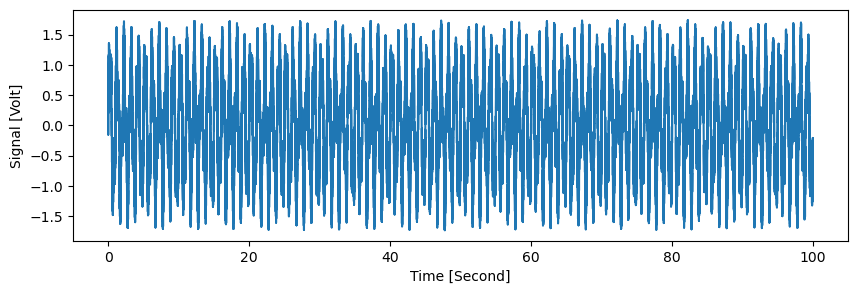
The data itself (sum of two sine signals with additive white noise)

signal1 = np.sin(2*np.pi*t)
signal2 = 0.5 * np.sin(2.8 * 2*np.pi*t)
noise = 0.5*(np.random.random(size=len(t)) - 0.5)
                         
data_array = signal1 + signal2 + noise

Data units for the data must be defined to store it in a flap data object.

data_unit = flap.coordinate.Unit(name='Signal', unit='Volt')

The data must also have coordinates associated. Since here the sampling is uniform (i.e. the coordinate is equidistant), only the start time and the increment is stored instead of storing the entire time vector. This is specified in a flap.coordinate.CoordinateMode object. The dimension_list parameter specifies the dimensions of the data associated with these coordinates.

For more details, see the corresponding sections of the User’s Guide and the API Reference.

coordinate_mode = flap.coordinate.CoordinateMode(equidistant=True)

data_coords = flap.coordinate.Coordinate(
    name='Time',
    unit='Second',
    mode=coordinate_mode,
    shape=[],
    start=t_start,
    step=dt,
    dimension_list=[0],
)

Now, the data object can be created with the associated data, data units and coordinates:

d = flap.DataObject(
    data_array=data_array,
    data_unit=data_unit,
    coordinates=data_coords
)

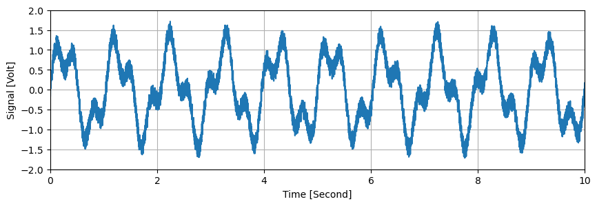
All flap features can now be used on this data object. Some examples:

Plotting:

plt.figure(figsize=(10,3))

d.plot(options={'All points': True})

plt.xlim(0,10)
plt.ylim(-2,2)
plt.grid()

plt.show()

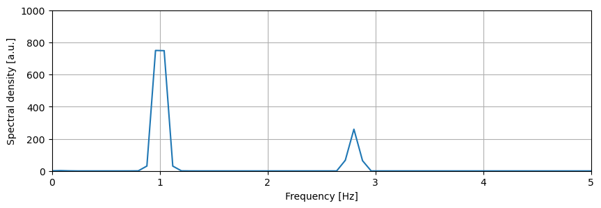
../../_images/403acbfa2bf8749888fb1fa0fae9b0c97c8cc74acb2205875fdc9bff70b93493.png

Auto-power spectral density:

d_apsd = d.apsd()

# Plot the APSD
plt.figure(figsize=(10,3))

d_apsd.plot()

plt.xlim(0,5)
plt.ylim(0,1000)
plt.grid()

plt.show()

../../_images/7ec98d78a9304c12e915e2b743f6783be14e3e9a9236d3156ca555e03d859edb.png

Saving and loading the data object as a pickled object:

d.save('test_save.pickle')

d_loaded = flap.load('test_save.pickle')

plt.figure(figsize=(10,3))
d_loaded.plot()
plt.show()

../../_images/7e690d54dac9dd22f7320d88a7047f6dd935545d71b7d0af36c419ed3c476e28.png

Creating FLAP data object directly from numpy array¶

Creating FLAP data object directly from `numpy` array¶