FLAP Version 1.21 User’s Guide¶

S. Zoletnik, D. Takács, HUN-REN Centre for Energy Research (https://www.ek.hun-ren.hu/en/home/)

zoletnik.sandor@ek.hun-ren.hu

Document version 1.72, 28 October, 2024

Introduction¶

The Fusion Library of Analysis Programs (FLAP) is a Python framework to work with large multi-dimensional data sets especially for turbulence data evaluation in fusion experiments. Data are stored in data objects together with coordinates and data names, thus the built-in plotting functions create figures with correct axes. The data set can be sliced to reduce dimensions and thus enable visualization of more than 2D data sets. FLAP is a modular package: data are read through modules which register themselves to the FLAP framework. This way data are read through a uniform interface by defining data source, experiment ID and data name. Also coordinate conversion is done by functions in the data source modules.

Obtaining and installing FLAP¶

Flap is available on GitHub at https://github.com/fusion-flap. There are multiple repositories. The core FLAP repository is named flap. Some data source packages are also stored here with names flap_xxx. See the Install for the installation steps of the main package. To use the data source packages, either refer to their README, or just clone the appropriate repository and add it to your Python PATH.

To test and see examples look at file tests/flap_tests.py in the flap repository. It contains various functions to test and demonstrate different functionalities. These functions are called at the end of the file where they can be one-by one switched on/off by changing True/False values. The test programs print some information and the contents the FLAP storage into the console and generate various plots with Matplotlib.

Additional illustrative examples are available in the Examples Gallery.

Configuration¶

FLAP can be adapted to the local environment using a configuration file. When flap is imported the default configuration file flap_defaults.cfg is loaded from the working directory. If the file is not found a warning is printed. A configuration file can also be read explicitly using the flap.config.read function.

The configuration file is a windows-style configuration file consisting of sections and elements. Sections start with their name in []. The elements follow on individual lines. The name of the element and the value is separated by =. Space can be used in both the section names and element names. Lowercase and uppercase characters are different. Usually names start with upper case but this is not a requirement. An example:

[PS]
Resolution = 1e3
Range = [1e3, 1e6]
[Module TESTDATA]
PS/Resolution = 100
Name = 'This is a string'

In the above example section “PS” contains two elements. Section “Module TESTDATA” refers to the TESTDATA data source module. The element PS/Resolution refers to the resolution element in the PS section and enables overriding section settings with module specific values.

All elements in a section can be read with the flap.config.get_all_section function. This returns a dictionary with keys referring to element names. The values are converted using the following rules:

True and Yes is converted to boolean True.
False and No is converted to boolean False.
An element enclosed in single or double quotes is handled as string (without the quotes).
Elements which can be converted to int, float or complex are interpreted accordingly.
An element enclosed in square brackets ([]) is interpreted as a list. List elements should be separated by commas. Each list element is interpreted using the same rules as one element of the section.
If all the above interpretation attempt fails the element is handled as string.

Options and defaults¶

Standard flap functions (like flap.data_object.get_data, flap.data_object.apsd, …) take an options keyword argument. A default options list is defined inside the routine, which contains all possible option keys understood by the function and default values for them. If no options are passed to the function these will take effect. The function might also be linked to a section in the configuration file. Options read from this section override the default options.

The above section defaults might be overridden with data source related values. The data object processed by the function might contain a data_source variable. If that is not None, configuration file elements in the section [Module <data_source>] are read and elements in the form {<section>}<parameter> are searched for. (Here <section> and <paramter> are names of a section and a parameter in it, respectively.) If such an element is found the respecting default parameter in <section> is overwritten with the value on the Module section.

As all possible options of the function are known from the default options dictionary it is allowed to abbreviate the option names in the function input options list up to the point where it matches only one key. (In the configuration file full option keys should be used.) This also means that any key in the default key list cannot be an abbreviation of another one. (E.g. ‘A’ and ‘A1’ are not allowed.)

This procedure is handled by the flap.config.merge_options function.

Data objects¶

Data objects are flap.DataObject class variables. They contain a multi-dimensional data array, an optional error array (symmetric or asymmetric), data name and data unit (in a flap.Unit object) and various information elements (info, history) which at present are not fully developed. A data object can optionally contain an exp_id variable (the type depending on the data module) describing the experiment ID from which the data originates from and the data source module name. An arbitrary number of coordinates are contained in the data object. This enables automatic plotting with proper axes and various calibrations. The coordinates are given as a list of flap.Coordinate objects is the dataobject’s coordinates attribute. The order in this list is irrelevant, as the dimension_list attribute in the coordinates defines how they map to the dataobject’s data_array. The data_source attribute contains the name of the data source (see below).

Data objects are normally created by the class constructor by giving the contents as its input arguments. It is also possible to omit some arguments and fill the elements in the data object later. Care should be taken that if the data array is given later, the data_shape element should also be filled.

Data sources¶

FLAP can make use of various data read modules which can be dynamically added to the package. Each package registers its data read and optional coordinate addition function in FLAP so as data are read using a single FLAP function called get_data. The parameters are the data source name, data name (interpreted by the data source module), experiment ID and additional coordinate information so as data can be limited to certain ranges or resampled in channels, time, etc. A single get_data call can read any number of measurement channels, there is an extended wildcard interpretation method which enables e.g. using Signal[2-28] to read signals from 2 to 28 into one data array. The module data read function can add as many coordinates to the data array as it desires to be useful. (See information on FLAP coordinates below.) Standard coordinates are Time, Signal name, Channel, etc. For information on writing a FLAP data source please see the appropriate section below.

Signal names¶

Signal names depend on the data source. There are data sources (e.g. MDS+) where signal names are arranged in a big tree and difficult to remember. To ease this a virtual signal name translation mechanism is provided. If used by the data source modul it allow setting up a virtual signal table where signals are translated to real signal names, which can be read from the DAQ system. This solution also allows for using extended wildcards in signal names.

An example virtual signal file is shown here:

[Virtual names]
ALL_SIGNALS = (S1,S2,S3,S30,S31,S32)
PART_SIGNALS1 = S[2-3]
PART_SIGNALS2 = S[30-31]
COMPLEX_SIGNAL = COMPLEX(S1,S2)
SIG(1234-2345) = DAC23
SIG(3455-4566) = DAC44

In this example reading ALL_SIGNALS will result in a DataObject containing signals S1…S3,S30,…S32. PART_SIGNALS1 will result in S2 and S3 while PART_SIGNALS2 will yield S30 and S31. COMPLEX_SIGNAL will yield a complex DataObject composed of two measured signals. The last two lines show examples how the signal name translation can be limited to certain shot number ranges.

The signal interpretation is fully recursive, lines in the file can link to other lines, complex signals can be listed to yield a DataObject with multiple complex signals, etc. It is the resonsibility of the programmer of a data source to make use of the above facility which is provided in the interpret_signals function.

Coordinates in FLAP¶

In the FLAP program package coordinates are stored with the data. This document describes the implementation of this feature.

Data storage and coordinates¶

Data are stored in an n-dimensional numpy array in the flap.DataObject class variable. This n-dimensional space we call data sample space. Different dimensions of the array are associated with primary coordinates, like sample number, channel number, or e.g. for simulated data x, y. However, these primary coordinates are often not useful and we need to make plots along physical coordinates. This can be handled by adding other coordinates to the DataObject. Also during processing some coordinates might be turned to others. An example is calculating power spectra. From a 2D measurement data with channel, time coordinates spectrum calculation creates another 2D array with channel, frequency as coordinates.

In order to be more general by coordinate we will consider all information related to the data, like measurement times, spatial locations, frequency, etc, especially what is variable for the data array elements. However, this is not necessarily the case, a single scalar coordinate value can be assigned to all elements as well. Coordinate information is not necessarily of numeric type, e.g. channel name can also be considered as coordinate information. On the other hand, other information (e.g. date of the measurement, measurement device configuration information) are not considered as coordinate but stored in the info dictionary of DataObject.

Multiple coordinate information may be present in the DataObject but all of them assign a value to all the array data elements. Storage of the coordinate information is designed by considering that a coordinate mostly changes along one or a few dimensions of the data, in a lot of cases coordinate values are equidistant but in special cases a coordinate value might change along all dimensions of the data array. This way the simple cases are described with minimal amount of data, while enabling even the most complicated case when data is practicably doubled by adding a randomly varying coordinate. Data processing, plotting is optimal if a coordinate changes along one dimension only.

Representation of coordinates¶

Coordinates have a name and unit, both described by a string. Standard names are ‘Channel name’, ‘Channel number’, ‘Signal name’, ‘Time’, ‘Sample’, ‘Device x’, ‘Device y’, ‘Device z’, ‘Device R’, ‘Device Z’, ‘Device phi’, ‘Flux r’, ‘Flux Theta’, ‘Flux phi’, ‘Image x’, ‘Image y’, ‘Frequency’, ‘Time lag’. Any other names and units can be used, but it is preferred to use the above where possible. The names are case sensitive as usual in Python. The type of the coordinate values is dependent on the coordinate type. E.g. ‘Sample’ is integer, ‘Time’ is either float or Decimal, ‘Signal name’ is string.

The following variables are defined in the Coordinate class, but not all of them are used in all definitions: name, unit, mode, shape, step, start, values, value_index, value_ranges, dimension_list. Unused variables are set to None.

Coordinates are not stored in the data matrix but each coordinate description is contained in a flap.Coordinate class object. Such an object describes the coordinate values in a d-dimensional rectangular coordinate sample space described by the shape variable what is a tuple of sample numbers \((s_1,s_2,\ldots, s_d)\) in each dimension, similarly to shape in numpy arrays. If shape has 0 elements it means that the coordinate value is constant and described by the values and value_ranges variables. The coordinate sample space is a subarray of the data sample space. As an example consider measurements on a 2D spatial mesh. At each measurement point a time signal is collected, thus the data sample space is 3D. If the 2D mesh is rotated relative to physical x,y coordinates then these physical coordinates will change on the 2D mesh. This way the coordinate sample space of x and y will be 2D, while the coordinate samples space for the time coordinate will be 1D.

The coordinate values are described in the coordinate sample space \([0 \ldots s_1-1, 0 \ldots s_2-1, \ldots, 0 \ldots s_d-1]\) in one of two ways.

If flap.Coordinate.mode.equidistant is False samples of the coordinate value are given on a regular or irregular grid in the coordinate sample space. The following cases are considered:
- If value_index is None and the shape of the coordinate sample space is identical to the corresponding subspace of the data sample space, then there is a one-to-one correspondence between data samples and coordinate samples. The coordinate values do not change along dimensions which are not in flap.Coordinate.dimension_list.
- If the two above shapes are different but value_index is None interpolation is done in the directions with different number of elements assuming that first and last samples match.
- If value_index is not None than coordinate samples are on an irregular grid. The coordinate sample locations are given in the value_index (\(d\) by \(N_{\mathrm{samp}}\)) array where \(N_{\mathrm{samp}}\) is he number of coordinate samples. The coordinates in the sample space are between 0 and \(s_i\) in the \(i\)-th dimension. The coordinate values are given in the 1D values array which has \(N_{\mathrm{samp}}\) elements. To calculate the coordinate value for the data array points a (multi-dimensional) interpolation is done between the sample coordinate system and the data sample coordinates.

When defining a non-equidistant coordinate giving the values attribute is not sufficient, the shape attribute also must be set. This tells whether the coordinate values can be directly mapped to the data samples or interpolation should be done. At present interpolating coordinates are not supported.

If flap.Coordinate.mode.equidistant is True then the coordinate sample space is assumed to be identical to the subspace of the data sample space selected by dimension_list. (flap.Coordinate.shape is not used.) The coordinates change linearly in each dimension: \(c=b+s_1 x_1 + \ldots s_d x_d\), where \(b\) is the start element of flap.Coordinate and \(s_i\) is the step size in dimension \(i\) of the data sample space. The \(s_i\) values are stored in the step element which is a \(d\) long 1D array.

The coordinate values may have a range which is either symmetric or asymmetric around the values. This can be considered either as an error of the coordinate or measurement range, and it is described by a value_ranges variable. If flap.Coordinate.mode.range_symmetric is True the range is symmetric around the coordinate values, otherwise there is a low and high range. For the equidistant coordinate description value_ranges is either a scalar or 2-element array depending whether the range is symmetric or asymmetric. For the non-equidistant coordinate description in the symmetric case value_ranges has the same shape as values, for the asymmteric case it is a dictionary with low and high keys. Each dictionary element has the same shape as values.

Mapping to data samples: the dimension_list attribute¶

The link between the coordinate sample space and the data sample space is established by the dimension_list element of flap.Coordinate. This has number of elements equal to the dimension of the coordinate sample space and each element contains the index of the related data sample space.

Getting coordinate values¶

The flap.Coordinate class has a data method which can be used to return the coordinate values for certain data array elements. As the data array shape is not know for the coordinate object a data_shape argument is needed. An optional index argument can be used to limit the calculation to certain elements. If the ‘Change only’ option is set only the coordinates along the changing data dimensions are returned.

The method returns three numpy arrays: the coordinate values and the coordinates at the lower and upper ranges. The shape of the arrays is set by the data_shape and index arguments and reflects the shape of the selected data array.

The flap.DataObject.coordinate('cname') method calls the flap.Coordinate.data method of the coordinate ‘cname’ by setting its data_shape argument to the data shape of the data object. Otherwise it is identical to the data method of flap.Coordinate.

Converting coordinates¶

Each data source may name a function in the registration process in the add_coord_func keyword variable. The add_coordinate() method of flap.DataObject gets coordinate name(s) (string, or string list) and options dictionary. It calls the function registered for the given data source with the data object, the new coordinate name(s) and options arguments. The function should add the named coordinate(s) to the data object or raise a ValueError. The function knows the experiment ID and other information about the data, therefore it should be possible to calculate the new coordinate.

Explanations and examples¶

The above definition is complex but it has a reason. It contains all possibilities from the most simple to the most complex. The coordinate descriptions are usually prepared in the data read module and the coordinate values accessed by the data() method of the Coordinate class, therefore the user should not take care of details of the coordinate description. Additionally, the most often encountered cases are very simple, difficulty arises only e.g. when random points are measured in time dependent flux coordinates at random time samples.

In the examples below we do not indicate the coordinate ranges, it can be simply added as described above.

Some typical situations:

Constant coordinate.

This is useful where e.g. a measurement is done with all measuring points in the Device z=const. coordinate. This constant can be entered in the DataObject description to be used later when e.g. mapping is done from device to flux coordinates.
```
shape = []
values = <z>
```
Independent equally spaced coordinates along each dimension of the data array.

In this case a coordinate is defined for each dimension of the data array. The definition of each coordinate contains a scalar start and a step value. The shape variable is one number, only the number of elements of shape is used showing that the coordinate description is 1D.
```
shape = 1
mode.equidistant = True
start = <start>
step = <step>
dimension_list = [0]
```
In the above example the coordinate changes along the first dimension of the data array.
Array of N temporal signals measured at N different points in the device coordinate space.

The data is stored in a 2D array, one dimension (0) is time, the other is channel. In this case a ‘Time’ coordinate is described with equidistant spacing as shown in the previous example. To describe the measurement spatial coordinates additionally to ‘Time’ 3 coordinates are entered in the coordinates list of the DataObject: ‘Device x’, ‘Device y’ and ‘Device z’. The description for the x coordinate is:
```
shape = N
mode.equidistant = False
values = <array with N elements of coordinate values>
```
The other two coordinates are entered similarly. The time vector and \(x,y,z\) coordinates of measuring channel i can be obtained from the d DataObject as:
```
time = d.coordinate('Time',(...,i))

x = d.coordinate('Device x',(i,0))
y = d.coordinate('Device y',(i,0))
z = d.coordinate('Device z',(i,0))
```
In this example it is also useful to additionally define a ‘Signal name’ and maybe a ‘Channel’ coordinate. Signal has normally string values (that is non-equidistant array, values is a list of strings).
Fast measurement signals at an array of spatial points mapped to a temporally slowly variable flux coordinate system.

The data are stored in a 2D array, 1-st dimension is channel, second is time. The data read routine enters the device coordinates into the DataObject. From this the flux coordinate calculation method generates the flux coordinates of the measurement points at a few time points (\(N_t\)) during the measurement time. 3 coordinates are added to DataObject, the three flux coordinates. For each coordinate the calculated values are put into a 1D array. The value_index will be a 2x\(N_t\) array, at each time point the channel number and the flux coordinate calculation time will be entered. The time is normalized to \((t-t_{start})/(t_{end}-t_{start}) (N_t-1)\). The shape variable is (\(N_{\mathrm{ch}}\), \(N_t\)), where \(N_{\mathrm{ch}}\) is the number of channels, mode is set to 0 and dimension_list to [0,1]. As in the channel direction the mapping is 1:1 from the coordinate sample coordinate and the data matrix coordinate no interpolation will occur. In the time direction interpolation will be done and the flux coordinates of each measurement channel will be interpolated values between the sparsely known flux coordinates. The ‘Time’ coordinate is entered as an equidistant coordinate description.

Data storage¶

Data object variables can be passed between functions in a program as any other variable. However, additionally to this FLAP contains a memory storage facility where data objects can be stored under a name and experiment ID. This enables loading and processing various data without the need of passing around a large number of variables. Data can be entered into the storage by the flap.add_data_object function and retrieved by flap.get_data_object. It is also possible to directly enter a data object from the flap.get_data function or all of the data processing functions.

Listing the content of FLAP storage¶

Function flap.list_data_objects can be used to list properties of the data objects in FLAP storage or in variable. From the storage data can be selected by name and exp_id (wildcards can be used). Data objects in variables can be listed by providing a list of the variables to the input of flap.list_data_objects. The data shape, properties and properties of coordinates are listed. The output string is returned by the function and printed on the screen unless the screen keyword argument is set to False.

Save/Load¶

Data objects can be saved to a file either from the FLAP data storage or from variables using the flap.save function. It can take a list of data objects or other variables or a list of strings and experiment IDs. In the latter case the data objects named by the strings and experiment IDs are loaded from FLAP storage before saving them. The save routine uses the pickle Python module to encode data. The file contains information whether data originates from FLAP storage or from variables. When data are loaded using the flap.load function they are returned as list of variables. If the data were saved from FLAP storage it can be entered there with the same names as well.

Data processing¶

The data processing routines are always available in two versions:

A method of the flap.DataObject class. The method does not change the original data object, rather returns the processed object.
A flap.<xxx> function, where <xxx> is the same name as the respective method in the flap.DataObject class. These functions read a data object from FLAP storage, call the method on them and store the result either the same or new name.

The function always have the same arguments as the method plus a few additional ones:

The first positional argument is the object name.
An exp_id keyword argument sets the exp_id of the data object. Default is '*', therefore exp_id need not be set unless there are data objects with the same name and different exp_id in the storage.
an output_name keyword sets the name of the resulting data object. If it is not set the result will be stored under the same name as the input.

Each processing function/method returns the resulting data object, therefore operations can be chained:

d.filter_data().apsd().plot()

Setting defaults for the processing method (see section Options and defaults) the exact parameters of the processing need not be written out in the most often used cases.

Slicing¶

Slicing means selecting certain elements in the data matrix and optionally taking their sum, minimum, maximum, or doing some other operation on them. Description of the slicing operation is based on coordinates. (Although originally it was foreseen to do slicing along data dimensions, this is not considered useful now.)

Slicing is performed with the slice_data method. In the slicing argument it takes a dictionary with keys referring to coordinates. The values describe how slicing is done. If the slicing dictionary has multiple keys the slicing operations are done sequentially, except a special case, see below. Summing is done after slicing. (If the slicing argument is omitted only summing is done.) Summing again defined by a dictionary where keys refer to coordinate names.

If the slicing coordinate changes only along one dimension of the data array slicing is done on the data along the associated dimension (see dimension_list). Other coordinates changing along this dimension are adjusted. It has to be noted that coordinate changes might result in changing from equidistant to non-equidistant type, which can cause more data in the data object. If only one data remains in the sliced dimension that dimension is dropped from the data and also coordinate dimension lists are adjusted correspondingly.

If the slicing coordinate changes along multiple dimensions the situation is more complex as shown in the 2D example below. Here \(x\),\(y\) are the original coordinates in a 2D array and \(R\) is some coordinate derived from them. The points are arranged in an \(x\)-\(y\) coordinate system. The orange lines indicate constant \(R\) contours. The two solid lines indicate slicing in the \(R\) coordinate, the red filled dots are the selected points. Selecting elements in the data in the range of a coordinate which changes in multiple dimensions means that the selected sub-array becomes non-rectangular. In this case the data along these dimensions will be flattened to 1D before slicing and the slicing operation will be done on the flattened dimensions.

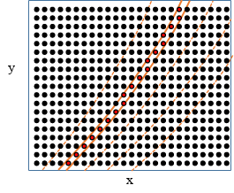
../_images/slicing_figure.png — Illustration of slicing example. Data in the original \(x\)-\(y\) coordinates, with constant-\(R\) contours.¶

To illustrate this further let us consider a 2D image. A polar coordinate system with origin in the center of the image is introduced and slicing is done in the radial coordinate. Selecting one radial area results in a 1D array. The angle coordinate will change non-monotonically on this. However, coordinates are corrected accordingly and it is still possible to plot as a function e.g. of polar angle.

Two basic slice types are distinguished:

Simple slice is an operation when a single interval or individual elements are selected along a coordinate. This is described above.
Multi-slice is an operation when multiple intervals are selected from the data. In this case the dimensions along which the slicing coordinate changes are flattened as described at simple slice and the intervals are selected. Two new dimensions are added to the data matrix. Along one the interval number, along the other the data index inside the intervals change. The interval data are distributed into these new dimensions and the original flattened dimension is removed. With this procedure it becomes possible to plot/sum data in individual intervals or across intervals.

Multi-slice is a complicated procedure and the above described scheme breaks down when multi-slice is intended on two coordinates which change on (partly) common dimensions. E.g. in the above described case of multi-slicing the data on an \(x\)-\(y\) grid to an \(r\)-\(φ\) grid poses problems. After multi-slicing with \(r\) one gets the two dimensions along and across the intervals. However, the multi-slicing along \(φ\) would flatten these into one dimension and create new intervals in \(φ\). To avoid this multi-slicing along multiple coordinates with common dimensions is done in one step and data are distributed into boxes arranged along each dimension. In case of \(n\) such slicing operations \(n+1\) dimensions are added with one dimension where the interval number changes along each coordinate and a single dimension where the sample index in one interval box changes. This case is not implemented yet.

After a multi-slice operation coordinates changing along the flattened dimensions are split into two coordinates: “Rel. <coord> in int(<sl_coord>)” and “Start <coord> in int(<sl_coord>)”. (Except for string coordinates where this is not possible and the original coordinate shape will be changed.) Here <coord> is the name of the coordinate and <sl_coord> is the name off the slicing coordinate. Also coordinates with names “Interval(<sl_coord>)” and “Interval(<sl_coord> index)” are added storing the interval number (along one coordinate) and the sample index in one interval.

If multi-slice operation results in different interval length, the dimension along the samples in the intervals will be set to the longest. Where data is shorter in one interval np.nan values will be filled in case of float data and 0 for int. (There is no integer Not-a-number value in Python.) In the coordinate matrix missing elements will be filled similarly to data.

Slicing can be described with the following objects:

For simple slice:

a. A Python slice or range object, to select a sequence of regularly spaced elements.

b. A scalar value or a list of scalars to select random elements.

c. A numpy array to select random elements.

d. flap.DataObject without error and with data unit.name equal to the slicing coordinate name.

e. flap.DataObject with the data unit.name not equal to the slicing coordinate, but one of the coordinate names equal to the slicing coordinate and the coordinate has no value_ranges.

f. flap.Intervals object with one interval.

Slicing can be one either by selecting the closest value or by linearly interpolating. The mode is set by the ‘Interpolation’ option (‘Closest value’ or ‘Linear’). Both the option name and option values can be abbreviated. If error is present for the data then it will also be interpolated the save way as data.

In cases 1a-e the data elements with closest or interpolated coordinates will be selected, while in case 1f all elements in the interval will be selected. In case a string type slicing coordinate matching between the slicing and the coordinate value is required instead of close match. (There is no sense in close match for strings.) However, extended wildcards can also be used, e.g. slicing='{Signal name':'TEST-*-3'} is a valid slicing expression.

For multi-slice:

a. flap.Intervals object with more than one interval.

b. flap.DataObject with data unit.name equal to the slicing coordinate. The error values give the intervals.

c. flap.DataObject with the data unit.name not equal to the slicing coordinate name but name of one coordinates equal to the slicing coordinate. The value_ranges select the intervals.

In the above cases automatically multi-slice mode is selected. This can be overridden by option ‘Slice type’ (values: ‘Simple’ or ‘Multi’). In this case the selected intervals will not be put into a new dimension but will be put in the same dimension one after the other. If a coordinate changed equidistantly along this dimension it will be modified to non-equidistant.

The summing input argument to the slice_data method can be used for processing the sliced data. This is also a dictionary with coordinate names as keys. Before processing the dimensions where the summing coordinate changes will be flattened. The values of the dictionary can be the following:

‘Sum’: Add all elements.
‘Mean’: Take the mean of all elements
‘Min’: Take the minimum of all elements
‘Max’: Take the maximum of all elements

As the result of the processing is a single value along the summing coordinate, this dimension will be removed from the data. After processing the data the coordinate changes will be done. In the case of ‘Sum’ and ‘Mean’ the mean of the coordinates of the summed data will be taken, while in the case of ‘Min’ and ‘Max’ the coordinate of the minimum or maximum value will be selected.

Examples¶

As an example we read all signals from the TESTDATA module for a 1 ms piece and store under name TESTDATA in flap storage:

d=flap.get_data('TESTDATA',name='*',
                options={'Scaling':'Volt'},
                object_name='TESTDATA',
                coordinates={'Time':[0,0.001]})

This results in a 3D data object where signals are arranged in row and column and the third dimension is time. ‘Time’, ‘Sample’, ‘Row’, ‘Column’ and ‘Signal name’ coordinates are supplied by the data read routine. Then we add spatial coordinates:

flap.add_coordinate('TESTDATA',
                    coordinates=['Device x','Device z','Device y'])

We can list the content of the data object using the flap.list_data_objects call, yielding the following ouput:

TESTDATA(exp_id:None) "Test data" shape:[15,10,1001]
Coords:
    'Sample'[n.a.](Dims:2) [<Equ.><R. symm.>] Start:  0.000E+00, Steps:  1.000E+00
    'Time'[Second](Dims:2) [<Equ.><R. symm.>] Start:  0.000E+00, Steps:  1.000E-06
    'Signal name'[n.a.](Dims:0,1, Shape:15,10) [<R. symm.>] Val:TEST-1-1, TEST-1-2, TEST-1-3, TEST-1-4, TEST-1-5, TEST-1-6, TEST-1-7, TEST-1-8, TEST-1-9, TEST-1-10, ...
    'Column'[n.a.](Dims:0, Shape:15) [<R. symm.>] Val. range:  1.000E+00 -  1.500E+01
    'Row'[n.a.](Dims:1, Shape:10) [<R. symm.>] Val:1, 2, 3, 4, 5, 6, 7, 8, 9, 10
    'Device x'[cm](Dims:0,1, Shape:15,10) [<R. symm.>] Val. range: -1.112E+00 -  6.657E+00
    'Device z'[cm](Dims:0,1, Shape:15,10) [<R. symm.>] Val. range:  0.000E+00 -  5.587E+00
    'Device y'[cm](Dims:, Shape:) [<R. symm.>] Val: 0.000E+00

The above list shows that Sample and Time changes along dimension 2 (3-rd dimension), Signal names change on the first tow dimensions, Column and Row changes on dimension 0 and 1, respectively. Device y does not change at all (emply dimension list) as the measurement channels are in the y=0 plane. Device x and y both change on dimensions 0,1 as the measurement matrix is inclined in the \(x\)-\(y\) plane.

A simple slice to select one signal looks like:

flap.slice_data('TESTDATA', slicing={'Signal name': 'TEST-1-3'},
                output_name='TESTDATA_slice')

The result is a 1D array:

TESTDATA_slice(exp_id:None) "Test data" shape:[1001]
Coords:
    'Sample'[n.a.](Dims:0) [<Equ.><R. symm.>] Start:  0.000E+00, Steps:  1.000E+00
    'Time'[Second](Dims:0) [<Equ.><R. symm.>] Start:  0.000E+00, Steps:  1.000E-06
    'Signal name'[n.a.](Dims:, Shape:1) [<R. symm.>] Val:TEST-1-3
    'Column'[n.a.](Dims:, Shape:1) [<R. symm.>] Val:1
    'Row'[n.a.](Dims:, Shape:1) [<R. symm.>] Val:3
    'Device x'[cm](Dims:, Shape:1) [<R. symm.>] Val:-2.472E-01
    'Device z'[cm](Dims:, Shape:1) [<R. symm.>] Val: 7.608E-01
    'Device y'[cm](Dims:, Shape:) [<R. symm.>] Val: 0.000E+00

Extended regular expressions can also be used. In the following expression 3 signals are selected, resulting in a 3x1001 data array:

TESTDATA_slice(exp_id:None) "Test data" shape:[3,1001]
Coords:
    'Sample'[n.a.](Dims:1) [<Equ.><R. symm.>] Start:  0.000E+00, Steps:  1.000E+00
    'Time'[Second](Dims:1) [<Equ.><R. symm.>] Start:  0.000E+00, Steps:  1.000E-06
    'Signal name'[n.a.](Dims:0, Shape:3) [<R. symm.>] Val:TEST-1-8, TEST-1-9, TEST-1-10
    'Column'[n.a.](Dims:0, Shape:3) [<R. symm.>] Val:1, 1, 1
    'Row'[n.a.](Dims:0, Shape:3) [<R. symm.>] Val:8, 9, 10
    'Device x'[cm](Dims:0, Shape:3) [<R. symm.>] Val:-8.652E-01, -9.889E-01, -1.112E+00
    'Device z'[cm](Dims:0, Shape:3) [<R. symm.>] Val: 2.663E+00,  3.043E+00,  3.424E+00
    'Device y'[cm](Dims:, Shape:) [<R. symm.>] Val: 0.000E+00

Arithmetic operations on data objects¶

Currently simple addition and multiplication is implemented between data objects and between data objects and scalar values. In case of operations between two data objects the resulting object will have only those coordinates which are identical in the two input objects.

Addition, subtraction¶

Data objects can be multiplied if their data geometry, and data name is identical. The error of the resulting data object identical to one of the inputs if the other has no error. If both have errors the resulting error is the square root of the squared errors. In case of asymmetric error the two error values are handled separately. If only one of the objects has Adding or subtracting a constant does not change the error

Multiplication¶

Data objects can be multiplied if their data geometry is identical. The data name and unit of the resulting data object will be the product of the two names/units or squared if the names/unit are identical. E.g. multiplying two data objects with ‘Volt’ units will result in ‘Volt^2’ unit.

If any of the data objects has no error the resulting data object will also have no error. For asymmetric errors the two value squares are added and square root taken to yield a symmetric error for the input object. The output (symmetric) error will be: \(\sqrt{\sigma_{1}^{2}\sigma_{2}^{2} + \sigma_{1}^{2}\mu_{2}^{2}{+ \sigma}_{2}^{2}\mu_{1}^{2}}\), where \(\sigma\) and \(\mu\) are the error and data value, respectively.

When multiplying with scalar the errors will be multiplied.

Data object conversions¶

The following methods of data object result in a modified object.

`real`¶

Returns a new data object with the data the real part of the original data. Coordinates and other properties are not modified.

`imag`¶

Returns a new data object with the data the imaginary part of the original data. Coordinates and other properties are not modified.

`abs_value`¶

Returns a new data object with the absolute value of the data. For complex data this is the amplitude.

`error_value`¶

Returns a new data object where the data is a copy of the error of the original data object and error is None.

Signal processing methods¶

Most signal processing methods/functions have a similar logic and interface. They operate on one or more “signals” which change along one coordinate, e.g. time. However, they can also be used to perform processing along any other coordinate, e.g. some spatial coordinate. The processing of these methods can be limited to a set of intervals in a coordinate. Two coordinates are distinguished. The processing coordinate is the one along which the processing is done, the selection coordinate is in which the intervals are defined. The common input arguments are the following:

coordinate: name of a coordinate along which the processing is done.
intervals: description of the intervals to which the operation is restricted. There are multiple possibilities:
- intervals is None. In this case no intervals are used, all data are processed.
- intervals is a dictionary. In this case only one key is expected to be present and the key is a coordinate name. The intervals are taken in this coordinate, which is not necessarily the same as the coordinate argument. The value of the dictionary is the interval description (see below).
- intervals is neither None, nor dictionary. In this case the intervals are selected along the processing coordinate and the intervals argument is the interval description.
The interval description can be any of the following:
- List of two numbers: describes a single interval between these tow coordinate values.
- flap.Intervals object. Can describe regular or irregular intervals.
- flap.DataObject. There are two cases similarly to slice_data. If the data name equals the selection coordinate then the data and errors are used as intervals. If the data name is different than the selection coordinate but one of the coordinates in the data object is identical to the selection coordinate then the coordinate values an value ranges are used as intervals.
options: any other parameter for processing.

Signal processing methods are the following:

`detrend`¶

This method subtracts a trend from the data along a given coordinate. If the coordinate is not set ‘Time’ is used.

`filter_data`¶

Filters the signals along a certain axis with one of numpy’s filters. For defining the filter it has a simplified interface capturing the important aspects.

`select`¶

Selects intervals from a signal either manually with the mouse or automatically based on some events. The selection can be limited to a set of intervals as in all signal processing methods. The intervals are saved in a data object. This can be used in other functions which use intervals, e.g. most of the data evaluation methods and slice_data. With slice_data, conditional averaging can be implemented.

Spectral and correlation analysis¶

These functions are somewhat similar to signal processing methods but processing can be done along multiple dimensions and interval selection has different meaning. The calculations can be done along coordinates, but only coordinates can be used which are equidistant and change along one dimension. This way there is one-to-one correspondence between coordinate values and array indices and we will use coordinate and dimension in the same way.

In the above subsections various methods are presented generally for multi-dimensional cases. At the end of the section a few practical examples will be shown to illustrate typical applications.

Auto Power Spectral Density (`apsd`)¶

The simplest spectrum calculation is Auto Spectral Power Density (power spectrum). Let us assume we have an \(N\)-dimensional data set \(D(x_{1},\ldots, x_{N})\) in which the time coordinate is changing along dimension \(n\). The power spectrum calculation is done with the apsd method which converts the time coordinate to frequency:

\[\begin{split} F\left( x_{1},x_{n - 1},f,x_{n + 1},\ldots, x_{N} \right) = \int_{}^{}{D\left( x_{1},\ldots x_{N} \right)\mathrm{e}^{2\pi f x_{n}}}\,\mathrm{d} x_{n},\\ P\left( x_{1},x_{n - 1},f,x_{n + 1},\ldots, x_{N} \right) = F\left( x_{1},x_{n - 1},f,x_{n + 1},\ldots, x_{N} \right) {F\left( x_{1},x_{n - 1},f,x_{n + 1}\ldots, x_{N} \right)}^{*}, \end{split}\]

where \(F()\) is the Fourier transform of \(D\) along dimension \(n\) and \(*\) means complex conjugate.

The apsd calculation of a multidimensional dataset can be interpreted as we have a multi-dimensional collection of time signals and the power spectrum is calculated for all of them in one step. This calculation assumes that statistically the signal is the same in the whole \(x_n\) coordinate. (It can be different in other dimensions, that is the power spectra can be different at different \(x_i\).) Sometimes this is not true and one intends to process only certain intervals or one would like to calculate an error for the correlations, thus intends to sample different regions and test the variability of the power spectrum. These processing regions in \(x_n\) can be selected with the interval keyword. The spectral calculation routines will limit calculation to these intervals and place identical length processing intervals into them for error calculation. The minimum number of processing intervals is set with the Interval_n option. The processing interval selection algorithm ensures that at least the required number of identical length intervals are selected. If Interval_n is large the algorithm will select smaller processing intervals but the number is fulfilled. If Interval_n is 1 and the intervals keyword is not set all data in the \(x_n\) dimension will be used. If Interval_n is not 1 the spectral calculation is done on all processing intervals separately and the final power spectrum will be the mean of the spectrum in the processing intervals. The error estimate of the spectral values will be the scatter of the values through the processing intervals divided by the square root of the number of processing intervals. The default value for Interval_n is 8, thus by default an error estimation will be obtained for the power spectrum. Selection of intervals in other than the calculation coordinates does not make sense as it would be identical to slicing. If that is intended the data should be sliced before calculation.

Spectral calculations can also be done in multiple dimensions. An example for two- dimensional power spectrum is the wavenumber spectrum. Assuming that \(x_i\) and \(x_j\) are two spatial coordinates in the data set the \(k\)-spectrum is

\[ P\left( x_{1},x_{i - 1},k_{1},x_{i + 1},\ldots, x_{j - 1} k_{2}, x_{j + 1}, x_{N} \right) = \int_{}^{}{D(x_{1},\ldots, x_{N})\mathrm{e}^{2\pi k_{1} x_{i}}} e^{2\pi k_{2} x_{j}}\,\mathrm{d}x_{i}\mathrm{d}x_{j}. \]

Again the wavenumber spectra (also called \(k\)-spectrum) is calculated in one step using the apsd function by specifying two coordinates \((x_i,x_j)\) for the calculation.

The coordinate after the apsd calculation can be wavenumber or frequency depending on the calculation coordinate. By default the result will be “Frequency” of the calculation coordinate is “Time” and “Wavenumber” if the calculation coordinate is not “Time”. This behaviour can be modified using the “Wavenumber” option.

It has to be noted that the cpsd method with a reference dataset does not calculate cross-power spectra within \(D\) and \(D_{\mathrm{ref}}\) only between functions in \(D\) and \(D_{\mathrm{ref}}\). To calculate cross-spectra within \(D\) no reference dataset has to be set.

Cross Power Spectral Density (`cpsd`)¶

Cross-power spectra are similar to auto power spectra but in the power calculation the Fourier transform of two different datasets are used. The second dataset is called the reference and set using the reference keyword argument. The calculation is done along one or more common coordinates. The number of elements and the coordinate values of the two datasets in the calculation dimensions should be identical. In this case the dimension of the resulting dataset will be the sum of the dimensions of the two original datasets minus the number of calculation dimensions. Let us consider two datasets \(D\) (with \(N\) dimensions) and \(D_{\mathrm{ref}}\) with \(M\) dimensions. We calculate the one-dimensional cross power spectral density along dimension \(x_i\) in \(D\) and \(y_j\) in \(D_{\mathrm{ref}}\):

\[\begin{split} F\left( x_{1},x_{i - 1},f,x_{i + 1},\ldots,x_{N} \right) = \int_{}^{}{D\left( x_{1},\ldots, x_{N} \right)\mathrm{e}^{2\pi fx_{i}}}\, \mathrm{d}x_{i},\\ F_{\mathrm{ref}}\left( y,y_{j - 1},f,y_{j + 1},\ldots, y_{M} \right) = \int_{}^{}{D_{\mathrm{ref}}\left( x_{1},\ldots, x_{M} \right)\mathrm{e}^{2\pi f y_{j}}}dy_{j},\end{split}\]

\[\begin{split} P\left( x_{1},x_{i - 1},x_{n + 1},\ldots, x_{N},y_{1},y_{j - 1},y_{j + 1},\ldots, y_{M}, f \right) = \\ = F\left( x_{1}, x_{i - 1}, f, x_{i + 1}, \ldots, x_{N} \right){F_{\mathrm{ref}}\left( y, y_{j - 1}, f, y_{j + 1}, \ldots, y_{M} \right)}^{*}. \end{split}\]

The number of dimensions of \(P\) is \(N+M-1\) and it contains the cross-power spectral density at all combinations of the \((x_k, k \neq i ; x_l, l \neq j)\) coordinate pairs. The reference dataset can also be identical to the first dataset, in this case the autopower spectra will be present in the diagonal of the cross-power spectrum dataset. Selection of processing intervals in the calculation coordinate and error calculation can be done similary to apsd.

Cross-correlation (`ccf`)¶

This method calculates cross-covariance or correlation between two datasets along one or more dimensions. Let us consider two datasets \(D\) (with \(N\) dimensions) and \(D_{\mathrm{ref}}\) with \(M\) dimensions. We calculate the one-dimensional cross-covariance along dimension \(x_i\) in \(D\) and \(y_j\) in \(D_{\mathrm{ref}}\):

\[\begin{split} K\left( x_{1},x_{i - 1},x_{n + 1},\ldots, x_{N},y_{1},y_{j - 1},y_{j + 1}\ldots, y_{M},\Delta \right) = \\ = \int_{}^{}{D\left( x_{1},x_{i - 1},x_{i},x_{i + 1},\ldots, x_{N} \right)}{D_{\mathrm{ref}}\left( y,y_{j - 1},x_{i} + \Delta,y_{j + 1},\ldots, y_{M} \right)}^{*} \, \mathrm{d} x_{i}. \end{split}\]

Similary to cpsd the number of dimension of the result will be \(N+M-1\). If \(D\) and \(D_{\mathrm{ref}}\) is one-dimensional than the result is a single cross-covariance function.

If the “Norm” option is set to True the calculated values are normalized with the autocorrelations to get the correlation function:

\[\begin{split} C\left( x_{1},x_{i - 1},x_{n + 1},\ldots, x_{N},y_{1},y_{j - 1},y_{j + 1}\ldots, y_{M}, \Delta \right) = \\ = \frac{K\left( x_{1},x_{i - 1},x_{n + 1}\ldots,x_{N},y_{1},y_{j - 1},y_{j + 1},\ldots,y_{M},\Delta \right)}{\sqrt{\int_{}^{}{D\left(\overline{x} \right){D\left( \overline{x} \right)}^{*}} \, \mathrm{d}x_{i} \int_{}^{}{D_{\mathrm{ref}}\left( \overline{y} \right){D_{\mathrm{ref}}\left( \overline{y} \right)}^{*}}\, \mathrm{d}y_{j}}} \end{split}\]

between all signals in two data objects. It does not calculate correlations in one object, to do this the second (reference) data object can be omitted. The number of dimensions of the resulting data object is the sum of the dimension number of the two data objects minus 1. The correlation function lag range and lag resolution can be set.

Typical applications¶

If d is a onedimensional dataset describing a signal vs time then d.apsd() (or flap.apsd(d)) returns the power spectrum. It is a one-dimensional dataset containing power as as function of frequency. The result is the same using the cpsd method and ccf returns the autocorrelation function.

In the second example we have temporal measurements at multiple spatial locations \(x\) and the data are stored in a two-dimensional dataset \(D(x,t)\). In this case apsd returns a two-dimensional dataset \(D(x,f)\), the power spectra at all spatial locations. cpsd will have 3 dimensions and will contain all cross-power spectra between various measurement locations. The ccf method will also return a 3-dimensional dataset containing the cross-correlation (or cross-covariance) functions between all signals.

In the third example we have an image stored in a two-dimensional dataset \(D(x,y)\). Applying apsd in 2D will result in \(P(k_x, k_y)\), the power density in the two-dimensional wavenumber vector space.

If we extend the image with a temporal dimension to 3D: \(D(x,y,t)\) (video data) we can calculate the power spectrum in each pixel by doing apsd along the time coordinate: \(P(x,y,f)\). Doing ccf in 2D along \(x\) and \(y\) results in \(C(\Delta_x, \Delta_y,t)\). This video shows the temporal evolution of the spatial correlation function.

Plotting¶

FLAP can generate various plots from data objects in a simple way using the plot method of flap.DataObject or the flap.plot function. A slicing and summing keyword argument allows to call the slice_data function from within the plot call so as a plot can be made of a slice of the data without the need to store the slice.

The following plot types are available:

plot_type	Data dimension	Data type	Description
‘xy’	1D	real	Plots data or coordinates as a curve.
‘xy’	1D	complex	Plots the real-imaginary or amplitude-phase as two separate curves.
‘scatter’	1D	real	Plots data as points.
‘scatter’	1D	complex	Plots the real-imaginary or amplitude-phase points as two separate plots.
‘multi xy’	2D	real	Plots each curve of the 2D data object above each other
‘grid xy’, ‘grid scatter’	3D	real	Plots xy plots on a 2D grid
‘image’	2D	real	Plots 2D data as image. Data on regular mesh is plotted as interpolated image, irregular as boxes around coordinate values.
‘contour’	2D	real	Contour plot.
‘anim-image’	3D	real	A series of ‘image’ plots, the third coordinate as time. It can also write an AVI file as output.
‘anim-contour’	3D	real	A series of ‘contour’ plots, the third coordinate is time. It can also write an AVI file as output.

Graphics are created using the matplotlib package but a FLAP plot may consist of multiple matplotlib plots. Each FLAP plot is identified by a flap.PlotID class variable returned by the plot function/method. It is possible to set the actual plot ID to a previously created one and thus add more data to an already existing plot.

The hierarchy and handling of graphics is the following:

Matplotlib may use multiple “figures”, each figure is a separate window in the computer.
A figure may contain multiple subplots created by the Matplotlib subplot, GridSpec and similar functions.
When the FLAP plot function/method is called it uses the current subplot setting and places its (possibly multiple) plots into the subplot area.
The PlotID of the last plot is remembered by flap, the next plot will be overplotted into the existing one. This is also true for multi-axis flap plots.
The plot_id keyword can be used in plot to specify an existing plot ID where the new one has to be overplotted. After the plot this plot ID becomes the current one.
The current plot ID can be changed with the flap.set_plot_id function as well.
If the plot destination area is changed by the Matplotlib subplot function overlapping plots will be erased. If the new area agrees with an existing one no erase will happen. This latter behaviour will be changed in new versions of Matplotlib.
If the plot type at an existing place is different from the requested new plot and error message will be raised. Setting the ‘Clear’ option in the plot call to True erases the previous plot.

FLAP uses the coordinate information in the data objects to create plots. The axes of the plots can be specified as axes=[ax1,ax2,...] where the list elements can be the following:

The string __Data__ means the data in the data object.
Any other string refers to a coordinate in the data object.
A data object means the data on that data object is used. This enables plotting as a function of another data object.
A constant means constant value for that coordinate.

The FLAP plot function/method has default plot types and plot axes for various types of data objects, therefore in many cases it is enough to use d.plot() to prepare a reasonable plot of the data object. If no axes are specified the first few coordinates in the data object and the data are used as default. E.g. for simple x-y plot the first coordinate and data are the default axes. When overplotting the default axes become the ones in the plot. This way if a signal is plotted as a function of sample number instead of time the next signal will be automatically overplotted as a function of sample. This also means that when overplotting a data object onto an existing plot where the data_name of the new data object does not match any axis on the plot all axes should be explicitly specified and forced (see below).

Axes and units are automatically placed on the plots. The language of the axes can be set in the call to plot in the ‘Language’ option. When overplotting the following rules apply for the axis title and unit:

Axes of the old and new plot are considered to be identical when both the names and units are identical.
If and old and new axis is not identical an error message is raised unless the ‘Force axes’ option is set to True.
When forced the following rules apply:
- If names or units are identical they will be preserved.
- If one of the names or units is not known ('' or None) the other will be used
- If none of the above applies the axis will have no name and/or unit.

The link to the data from which the plots were created is saved in plotID and this in following versions on FLAP it should be possible to regenerate the plot, erase one of the data objects from it and possibly increase plot resolution when the ‘All points’ option is not set.

Writing a data source module¶

A data source module differs from a normal Python module in the in that it can provide a few functions for the FLAP framework. These are the following.

Reading data into FLAP¶

In order to implement data read into FLAP the module should provide a function with the following input arguments:

def get_data(exp_id=None,
                data_source=None,
                data_name=None,
                no_data=False,
                options=None,
                coordinates=None)

The name of the function is irrelevant. The input arguments are the following:

`exp_id`¶

The experiment ID that is shot number or any other numeric or string describing the particular experiment from which the data is requested.

`data_source`¶

The data source name. This is forwarded from the general flap.get_data() function. It can be used by the module get_data function to identify various subtypes of the same module.

`data_name`¶

Name of the data requested. This is a string or list of strings. The strings may contain Unix-style wildcards like CH[1-8] but also an extended wildcards can be used like CH[1-23]. This allows reading an arbitrary number and configuration of measurement channels. At present only one [...] wildcard can be used in a name.

`no_data`¶

If False then no data should be returned, only the coordinates filled. In this case it is necessary to set the data_source argument in flap.DataObject to indicate what the shape of the data would be. If this is not set the coordinate ranges cannot be determined. If the data_array is set in flap.DataObject the data_shape need not be set it will be determined from the shape of the data array.

`options`¶

A dictionary of options. No make use of options in the configuration file and abbreviation of options follow the description below.

`coordinates`¶

This dictionary may contain names of coordinates as keys and flap.Coordinate objects as values which can precisely define the coordinate ranges from which the data should be read through the values and value_ranges in the flap.Coordinate object. As a simplification the c_range element of the flap.Coordinate object gives a simple range.

Any number of coordinates can be added to the flap.DataObject.coordinates list. However, there should be at least as many coordinates as data dimensions otherwise the data object might be unusable for processing. In a standard case there is a coordinate describing each dimension of the data object, e.g. ‘Image x’, ‘Image y’, ‘Time’ for a series of images. More coordinates can be added, e.g. a ‘Sample’ coordinate with integer step and start value is often useful additionally to a ‘Time’ coordinate for long data sequences where the float representation of the Time data is not exact enough. The returned data object is checked for consistency by the flap.get_data() function.

The order of coordinates is arbitrary, but for default plotting the first few coordinates are selected, therefore is useful to check which are the default coordinates for the given dimensional data object.

Return value¶

The return value should be a flap.DataObject.

Using options¶

To make use of options in the configuration file and option abbreviation the following should be provided in the data read function:

A dictionary should be created with all possible options and their default values.

The flap.config.merge_options() function should be called the following way:

_options = flap.config.merge_options(default_options,
                                     options,
                                     data_source='DATASOURCE')

In the above call ‘DATASOURCE’ should be replaced with the data source name used in registering the data read function (see below). default_options is the default options dictionary and options is the options dictionary received by the get data function. In the above example the merge_options function reads entries from the configuration file section ‘Module DATASOURCE’ and all the entries which has no {xxx} at their beginning are added (or replaced) to the options list received in the default options argument. This means function defaults are replaced by configuration defaults. Finally the dictionary keys in the options arguments are checked whether they can be interpreted as abbreviation of only one option and if is fulfilled their value is entered into that options. This overwrites both function and configuration file defaults with input options. The resulting options dictionary is returned by the function. It should be named differently then the options input to the data read function to avoid overwriting the input argument. The _options dictionary should be used in the data read function after merging all options. This procedure is not compulsory but it should be done if configuration file options and option abbreviations are to be used.

Adding coordinates¶

An optional function can also be provided by the module if it is capable of calculating additional coordinates to the ones returned in the data read function. For e.g. some derived spatial coordinates or flux coordinates can be added to an already existing data object with the following function:

def add_coordinate(data_object,
                   coordinates=None,
                   exp_id=None,
                   options=None)

This function takes a flap.DataObject and adds new coordinates named in the string list “coordinates”. The arguments:

`data_object`¶

The input data object.

`coordinates`¶

A list of strings describing the requested new coordinates. In response the function should add these coordinates to the data object or raise an error.

`exp_id`¶

If for the coordinate calculation another experiment ID should be used this argument is set and used instead of the exp_id in the data object. This can be the situation e.g. when no calibration data is available for the original experiment.

`options`¶

A dictionary of options.

To make use of these tow functions in the flap environment the module should register them. The module should define a function named register the following way:

def register(data_source=None):
    if (data_source is None):
        data_source = 'DATA_SOURCE_NAME'
    flap.register_data_source(data_source,
                              get_data_func=get_data,
                              add_coord_func=add_coordinate)

The two functions in the get_data_func and add_coord_func are the two functions described above. This register function will be called when the module is used. (See in the next section.)

The ‘DATA_SOURCE_NAME’ string should be replaced by the desired data source name in FLAP. If the data_source input is not given the data source will be registered under the default name ‘DATA_SOURCE_NAME’, otherwise the calling program can register under a different name. This is useful if the same module is used for different data sources, e.g. a generic mds+ module for different experiments.

Using data source modules¶

To make use of a data source module it should be first imported in the user program as any other module. The data read and coordinate add functions are integrated into FLAP by calling the register function of the data source. In the example below we will use module name testdata and data source name ‘TESTDATA’.

Reading data¶

import testdata
testdata.register()

print(flap.list_data_sources())

d=flap.get_data('TESTDATA',
                exp_id=12345,
                name=['Signal-1','Signal-[20-23]'],
                options={'Scaling':'Volt'},\
                coordinates={'Time': [1,3]},
                object_name='TESTDATA_SIGNALS')

The above example code imports the testdata module and registers it in FLAP. The flap.list_data_sources function lists all actually registered data sources. The flap.get_data() function is the general data read interface in FLAP. In the example it reads from the ‘TESTDATA’ data source the data named ‘Signal-1’, ‘Signal-20’, … ‘Signal-23’ in the time interval 1-3s. The resulting data object will be stored in FLAP storage under name ‘TESTDATA_SIGNALS’ and also returned by the function. In the options it is requested to scale the data to volts.

When the flap.get_data() function is called it first determines whether the requested data source is registered. If it is then the data read function of the module is called with the exp_id, name, options, coordinates arguments. If the coordinates argument is a dictionary as in the above example then it is converted to a flap.Coordinate object and the range ([1,3] in the example) is entered in the c_range field of it. This coordinate is passed to the module data read function. If in the coordinates arguments already flap.Coordinate objects are listed then they are passed without modification. When the module data read function returns the data object it is stored in FLAP storage if an object name is named. The shape, contents, coordinates of the data object is fully determined by the module data read function.

Requesting new coordinates¶

In the simplest form new coordinates can be requested for data object d the following way:

d.add_coordinate(coordinates=['Device x','Device y'])

This call requests the module which created the d data object to add new coordinates named ‘Device x’ and ‘Device y’. The add_coordinate method also has a data_source, exp_id argument so as different data source or experiment can be used for coordinate calculation than the ones used for reading the data. This is useful e.g. when a separate flux coordinate mapping module is defined. It is also possible to add coordinates directly to a data object in FLAP storage:

flap.add_coordinate('TESTDATA_SIGNALS',
                    coordinates=['Device x','Device y'])

FLAP Version 1.21 User’s Guide¶

Introduction¶

Obtaining and installing FLAP¶

Configuration¶

Options and defaults¶

Data objects¶

Data sources¶

Signal names¶

Coordinates in FLAP¶

Data storage and coordinates¶

Representation of coordinates¶

Mapping to data samples: the dimension_list attribute¶

Getting coordinate values¶

Converting coordinates¶

Explanations and examples¶

Data storage¶

Listing the content of FLAP storage¶

Save/Load¶

Data processing¶

Slicing¶

Examples¶

Arithmetic operations on data objects¶

Addition, subtraction¶

Multiplication¶

Data object conversions¶

real¶

imag¶

abs_value¶

error_value¶

Signal processing methods¶

detrend¶

filter_data¶

select¶

Spectral and correlation analysis¶

Auto Power Spectral Density (apsd)¶

Cross Power Spectral Density (cpsd)¶

Cross-correlation (ccf)¶

Typical applications¶

Plotting¶

Writing a data source module¶

Reading data into FLAP¶

exp_id¶

data_source¶

data_name¶

no_data¶

options¶

coordinates¶

Return value¶

Using options¶

Adding coordinates¶

data_object¶

coordinates¶

exp_id¶

options¶

Using data source modules¶

Reading data¶

Requesting new coordinates¶

`real`¶

`imag`¶

`abs_value`¶

`error_value`¶

`detrend`¶

`filter_data`¶

`select`¶

Auto Power Spectral Density (`apsd`)¶

Cross Power Spectral Density (`cpsd`)¶

Cross-correlation (`ccf`)¶

`exp_id`¶

`data_source`¶

`data_name`¶

`no_data`¶

`options`¶

`coordinates`¶

`data_object`¶

`coordinates`¶

`exp_id`¶

`options`¶